Tutorial

Relevant imports

import matplotlib.pyplot as plt
import numpy as np
import pyforfluids as pff

Definition of the model to be used

model = pff.models.GERG2008()

Fluid’s initial state

temperature = 250  # Degrees Kelvin
density = 1  # mol/L
pressure = 101325  # Pa
composition = {'methane': 0.9, 'ethane': 0.05, 'propane': 0.05}  # Molar fractions

Definition of the fluid

The properties will be calculated at the moment of the object definition.

fluid = pff.Fluid(
    model=model,
    composition=composition,
    temperature=temperature,
    density=density
)

Pressure as an init variable

Pressure can be used as an initial variable, in this case the method fluid.density_iterator will be called internally to find the root of density at the given pressure, since all models use density as an independent variable instead of temperature.

This can lead to trouble since multiple roots can be obtained in the equilibrium region!

fluid = pff.Fluid(
    model=model,
    composition=composition,
    temperature=temperature,
    pressure=pressure
)

Accessing properties

Properties are stored in the Fluid attribute Fluid.properties as a dictionary, they can either be accessed that way or by calling them directly from the fluid.

All the properties are expressed in International System units, except for density that’s expressed in [mol/L]

fluid.properties

{'density_r': 9.442772800175154,
 'temperature_r': 207.1068112975803,
 'delta': 0.005162295708090389,
 'tau': 0.8284272451903212,
 'ao': array([[-3.47583079e+01,  0.00000000e+00,  0.00000000e+00],
        [ 1.93712266e+02, -4.99964400e+01,  0.00000000e+00],
        [-3.75244420e+04, -5.41251465e+00,  0.00000000e+00]]),
 'ar': array([[-0.0041676 ,  0.        ,  0.        ],
        [-0.80651578, -0.0108937 ,  0.        ],
        [ 0.31041621, -0.00769256, -2.10957546]]),
 'z': 0.9958365270355344,
 'cv': 30.928532328981273,
 'cp': 39.39441402789975,
 'w': 380.3778978355614,
 'isothermal_thermal_coefficent': -0.2725846588975132,
 'dp_dt': 0.4072695321069243,
 'dp_drho': 2061.3266554120955,
 'dp_dv': -4.898145216338861,
 'p': 100903.24995863381,
 's': -55.41564180556873,
 'u': -86111.8177689482,
 'h': -84041.85403879466,
 'g': -70187.94358740246,
 'jt': 0.00035980611360190225,
 'k': 1.2633809737968698,
 'b': -0.08557993798318263,
 'c': 0.003479888600305259}

fluid['cv']

30.928532328981273

State changes

A fluid thermodynamic variable can be changed by using the methods:

• Fluid.set_temperature

• Fluid.set_composition

• Fluid.set_density

• Fluid.set_pressure

When a property is changed, the properties are not re-calculated, so it’s a must to call the method Fluid.calculate_properties. This is intended to avoid useless calculations if two or more variables are to be changed. In the case of a pressure change Fluid.density_iterator will be called!

fluid.set_temperature(280)
fluid.set_density(2)

fluid.calculate_properties()

fluid['cv']

34.71399971808808

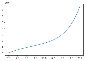
Calculating isotherms

Isotherms at the fluid temperature can be calculated along a density range with the method Fluid.isotherm. This will return a dictionary equivalent to the Fluid.properties one, but each value will be a list instead of a single value.

density_range = np.linspace(0.001, 20, 100)
isotherm = fluid.isotherm(density_range)

isotherm['cv'][:5]

[33.34361845195672,
 33.48240604268746,
 33.622421620895594,
 33.76309070522664,
 33.903893177656855]

plt.plot(density_range, isotherm['p'])
plt.show()